This document summarizes how I analyze raw Illumina data on an Apple Mac Pro. I often refer often to the analysis of strain TT26511. The page you are reading was exported as HTML from my electronic notebook, created using the application Notebook ($50, http://www.circusponies.com/). Notebook is an excellent way to keep track of the many steps and copious data generated during data reduction.

			Aside from Microsoft Excel, the remaining software described in this primer is free and in the public domain (or a component of the OS X operating system).

			When you installed the latest version of OS X on your computer, you probably did the easy install, in which case, you should do the following:

			Illumina data reduction requires commands run in a terminal window provided by the Terminal application (/Applications/Utilities). You will need to be familiar with the following when using this program. All are intrinsic parts of the underlying Unix foundation of OS X.

			Terminal commands in this primer are usually prefixed with "$ " to indicate the standard terminal prompt. This symbol should not be copied when trying out the command.

			Some of my tools are written in Python. No knowledge of this language is required to run them, but it is important that the version number be 2.7 or higher and less than 3.0. The latter is actually a different language and is incompatible with my setup.

			I use the "maq" suite of DNA analysis programs to manipulate Illumina data. They were recommended highly by Yong Lu in Fritz Roth's lab and have proven invaluable in my work. Maq can be downloaded here. To learn more about it, consult the manual.

			Unix variables can be created which will allow easy access to directories, databases, etc.

			The following illustrates the bash code for setting variables pointing to data directories in the analysis of TT26511.

			To see the value of a Unix variable, prefix the variable name with "$". In the following examples, "echo" is the bash word for "print":

			The Unix command for "connect to directory" is "cd". To go to folder /Users/kofoid/projects/inverted_duplications/Solexa/3_5_12/tt26511, do the following:

			To be useful, command lines creating variables must be stored in a bash startup file, which is loaded whenever you begin a session with Terminal. I use a file called ".bash_temp" in my home directory (Unix abbreviation "~"), and insert the following line in the startup file "~/.bash_profile" to call it:

			These steps convert the data to forms which allow easy construction of read-depth profiles, SNP discovery, description of rearrangements, etc.

			The raw data you receive can be in any one of a number of formats, depending on the kind of preprocessing done by your sequencing facility. My sample page assumes a file in zipped Illumina fastq format, segmented into multiple files. The following steps uncompress, merge and convert the data into the Sanger fastq format used by maq:

			At this point, you should check the data for suffices "#0/1" or "#0/2" at the ends of descriptors for left or right reads, respectively. Many facilities remove these during preprocessing.

			Convert fastq to fasta, which will be used to build a Blast database (and can also be used directly as a FastA database). Again, you will have to substitute the correct descriptor prefix for "@DJB775P1":

			Convert fastq to the binary format, "bfq", used by many maq programs:

			You can search your data for specific targets using a local copy of the NCBI Blast program, which can be downloaded here. This also installs a variety of tools, including "makeblastdb" which can be used to create a Blast database from fasta-formatted data:

			Note that I also created a Unix variable which points to the location of the database, and stored the line creating it in my .bash_temp file (see above).

			Blast front end

			Typical Blast search using the above variable for the database:

			Everything derived from the raw data files is really big! You should have a backup strategy for the base fastq files created after expanding the compressed raw files. If you use Time Machine (TM), then leave the fastq files in the current directory. Because you will never change them, TM will back them up once and never again, which is good. You should also copy them to a portable hard disk which you can keep off site (or at least in another room). Your sequencing facility will probably keep the original files for a few weeks to months, but don't rely on them to store your data forever.

			All the derived files (Sanger fastq, fasta, bfq, blast, etc.) can be recreated if lost, and would only take up unnecessary space in the TM archive.  Notice that when I did the sol2sanger step, the Sanger fastq files were placed in a different directory, $dtt26511, after which I moved to that directory ("cd $dtt26511"). All other big files were also stored there. I have instructed TM to not backup anything in folders beginning with "d", which indicates "don't archive".

			Here, we finally do the good stuff.

			Remember, we're in the "big file" directory. First, I create a subdirectory for chromosomal stuff, "dsty", and move into it:

			Now I run a workhorse script, "sol", which does all the rest of the work and spits out a plot, a histogram file readable by Excel, and some searchable "view" files. The code is here. This particular script calls several maq programs, and ultimately generates a plot by calling a script "rdplot", the code for which is here.

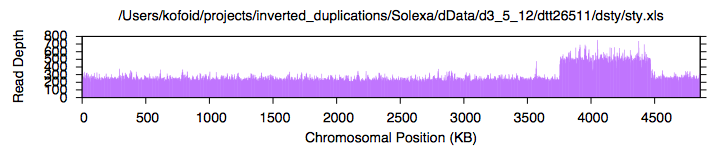
			If "sol" runs successfully, you will see some amusing lines of information scroll up in the terminal window, and eventually a plot will appear in an AquaTerm graphic window which looks something like this:

			In general, I have tried to avoid using any proprietary software. However, in the sample page for TT26511, you will notice some statistics regarding read depth, such as "overall read depth", "standard deviation of read depth", "amplification ratio", etc. My quick-and-dirty method for calculating these uses Excel. Eventually, I'll write a script to do this, but don't hold your breath.

			"sol" produces a file with extension ".xls" which contains the binned data necessary to generate the above plot, It can also be used to calculate statistics in Excel.

				Here is a typical Excel file used for this purpose:

				Positional normalization is a method for removing much of the noise from a read-depth plot. To use this technique, you must also have sequenced an unselected parental control strain along with the test strains. Here is an Excel file with normalization:

				find-anamo

			getfv

			cap3

			fasta

			This discussion assumes that your bioinformatic software is running on a server under OS X,  always kept on, and configured for file sharing as follows:

			From the client machine (an OS X computer remote from the server), link to the server using "Finder/Go/Connect to Server..."

			Open the Terminal program and connect to the server as follows:

			On a couple of occasions, I have written master scripts which automate everything, from raw data to the final profile. Invariably, they screw up, often with loss of data. The lesson: Don't try to do too much in a single step! Similarly, try to convince your sequence facility to keep your raw data on their server as long as possible, just in case you have to fetch it again.

			Many of these procedures and tools are in flux and being improved. I'm happy to hear comments and suggestions, especially about improvements in my code.